Life Science
Time-resolved Fluorescence
Measuring the fluorescence lifetime provides insights into the excited state dynamics of an emitter
The fluorescence (or in general photoluminescence) lifetime is characteristic for each fluorescent or phosphorescent molecule and can thus be used to characterize a sample. It is, however, also influenced by the chemical composition of its environment. Additional processes like Förster Resonance Energy Transfer (FRET), quenching, charge transfer, solvation dynamics, or molecular rotation also have an effect on the decay kinetics. Lifetime changes can therefore be used to gain information about the local chemical environment or to follow reaction mechanisms.
 Contact us
 Time-Correlated Single Photon Counting (TCSPC) is used to determine the fluorescence lifetime. In TCSPC, one measures the time between sample excitation by a pulsed laser and the arrival of the emitted photon at the detector. TCSPC requires a defined “start”, provided by the electronics steering the laser pulse or a photodiode, and a defined “stop” signal, realized by detection with single-photon sensitive detectors. The measurement of this time delay is repeated many times to account for the statistical nature of the fluorophores emission. The delay times are sorted into a histogram that plots the occurrence of emission over time after the excitation pulse.
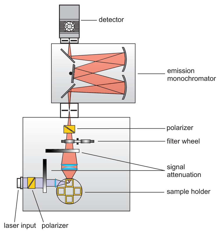
Consequently the essential components of a set-up for measuring fluorescence lifetimes are:
- pulsed laser source (diode laser, LED or multi-photon excitation)
- single photon sensitive detector
- means of separating fluorescence signal from excitation light (monochromator or optical filters)
- TCSPC unit to measure the time between excitation and fluorescence emission
Related technical and application notes:
PicoQuant offers the following systems capable of fluorescence lifetime measurements
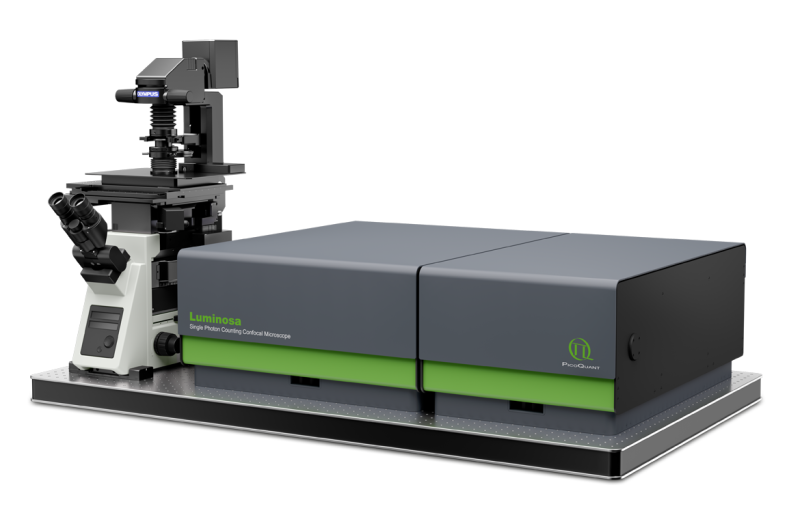
 Luminosa
Single Photon Counting Confocal Microscope
Luminosa combines state-of-the-art hardware with cutting edge software to deliver highest quality data while simplifying daily operation. The software includes context-based workflows for FLIM, FRET, and FCS, which allow the users to focus on their samples. Tight integration of hardware and software enable automated routines, e.g., for auto-alignment or laser power calibration, which increase ease of use as well as reproducibility of experiments. Still, an open mode of operation is available for full access to every optomechanical component via software.
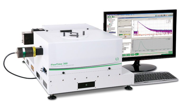
 FluoTime 300
High performance fluorescence lifetime spectrometer
The FluoTime 300 "EasyTau" is a fully automated, high performance fluorescence lifetime spectrometer with steady-state and phosphorescence option. The system features an ultimate sensitivity with a record breaking 24.000:1 Water Raman SNR. The FluoTime 300 contains the complete optics and electronics for recording fluorescence decays by means of Time-Correlated Single Photon Counting (TCSPC) or Multichannel Scaling (MCS). The system is designed to be used with picosecond pulsed diode lasers, LEDs or Xenon lamps. Multiple detector options enable a large range of system configurations. The FluoTime 300 can be used to study fluorescence and phosphorescence decays between a few picoseconds and several seconds
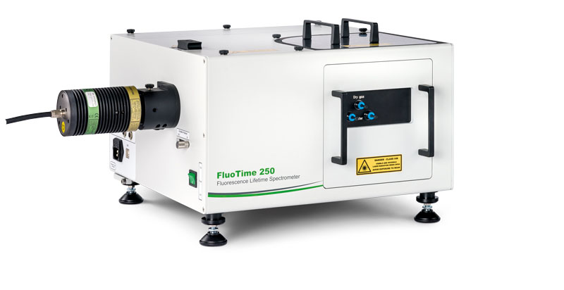
 Compact and modular fluorescence lifetime spectrometer
The FluoTime 250 integrates all essential optics and electronics for time-resolved luminescence spectroscopy in a compact, fully automated device. This spectrometer is designed to assist the user in carrying out routine as well as complex measurements easily and with high reliability thanks to fully automated hardware components and a versatile system software featuring wizards providing step-by-step guidance.
The following core components are needed to build a system capable of time-resolved fluorescence measurements, which are (partly) available from PicoQuant:
- Laser drivers
- Laser or LED heads
- Photon Counting Detector
- TCSPC and MCS Electronics
- Analysis software
- Monochromator
- Focussing and collection optics
Fluorescence lifetime measurements have a multitude of possible applications depending on how the lifetime information is interpreted, such as:
- Identify or separate species by their fluorescence lifetime
- Monitor changes in the environment
- Study protein folding or signaling pathways
- Detect singlet oxygen for photodynamic therapy
- Study membrane rigidity or enzyme/substrate interactions
- ...
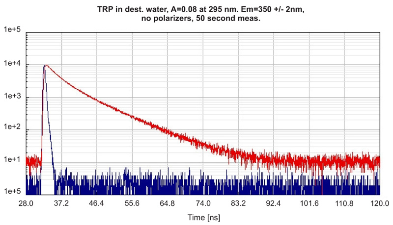
Recording the time-resolved fluorescence spectrum of L-Tryptophane in water
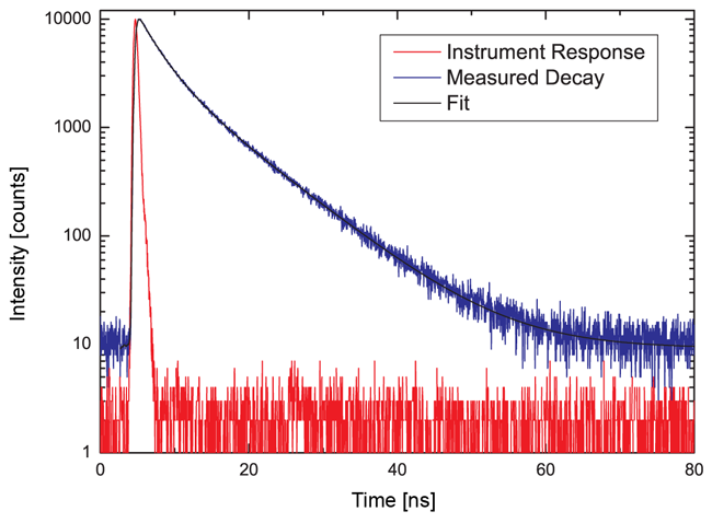
 A solution of L-Tryptophane in water (HPLC quality) was excited at 300 nm. The collected emission passed a monochromator set to 350 nm with 4 nm bandpass. The measured instrument response function (IRF) has a FWHM of 600 ps and 1.5 million counts were collected within 50 seconds measurement time. No polarizers were used in the set-up.
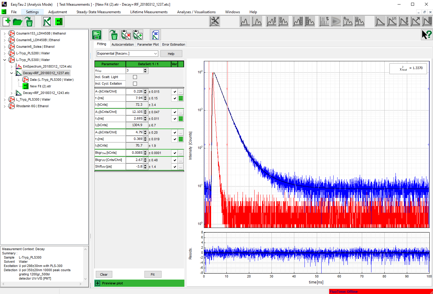
 As can be expected for L-Tryptophane the decay is best described by a triple exponential decay funciton. The picture shows the IRF (red), the measured decay (blue) and the result of the fit (black). The recovered lifetimes are 0.37 ± 0.02 ns , 2.69 ± 0.01 ns and 7,94 ± 0.015 ns. The errors were calculated using bootstrap error analysis.
- FluoTime 300
- Excitation: PLS 300, 10 MHz repetition rate
- Analysis: EasyTau 2
Time-resolved fluorescence measurement of Coumarin 152 in ethanol
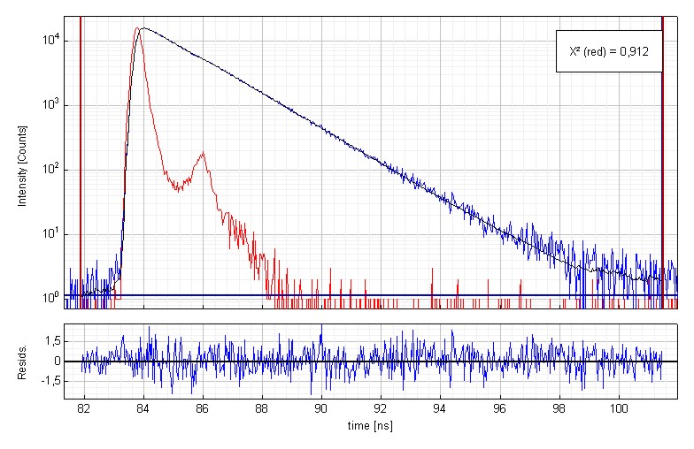
, IRF (red), and fitted curve (black)") Time-resolved fluorescence lifetime measurement of Coumarin 152 (3·10-7 molar) in ethanol. The plot shows the measured Instrument Response Function (red), the sample decay (blue) and the fitted decay. The fluorescence lifetime is 1.59 ns. An excellent chi-square of 0.912 and the residual trace demonstrate the quality of the fit.
Time-resolved fluorescence lifetime measurement of Coumarin 152 (3·10-7 molar) in ethanol. The plot shows the measured Instrument Response Function (red), the sample decay (blue) and the fitted decay. The fluorescence lifetime is 1.59 ns. An excellent chi-square of 0.912 and the residual trace demonstrate the quality of the fit.
Set-up:
- FluoTime 100
- Excitation: 405 nm, 20 MHz repetition rate
- Analysis: FluoFit (replaced by EasyTau 2)
Determining the fluorescence lifetime of Oxazine 1 in water
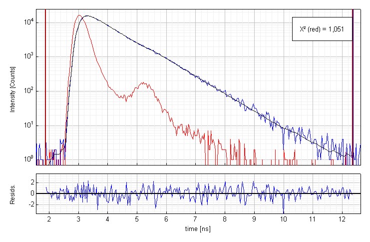
 with IRF (red) and fitted decay curve (black)") Time-resolved fluorescence lifetime measurement of Oxazin 1 (1·10-6 molar) in water. The plot shows the measured Instrument Response Function (red), the sample decay (blue) and the fitted decay. The fluorescence lifetime is 799 ps. An excellent chi-square of 1.051 and the residual trace demonstrate the quality of the fit.
Time-resolved fluorescence lifetime measurement of Oxazin 1 (1·10-6 molar) in water. The plot shows the measured Instrument Response Function (red), the sample decay (blue) and the fitted decay. The fluorescence lifetime is 799 ps. An excellent chi-square of 1.051 and the residual trace demonstrate the quality of the fit.
Set-up:
- FluoTime 100
- Excitation: 635 nm, 20 MHz repetition rate
- Analysis: FluoFit (replaced by EasyTau 2)
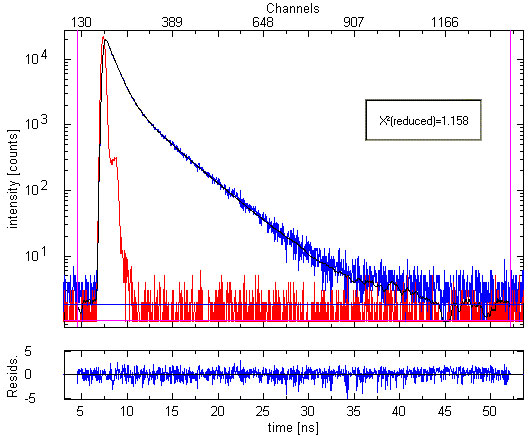
Investigating a mixture of Oxazine 1 and Oxazine 4 via time-resolved fluorescence spectroscopy
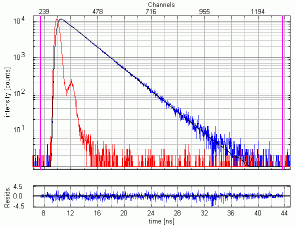
 with fit (black) and IRF (red)") Fluorescence decay measurement of Oxazine 1 with a trace amount of Oxazine 4 (10-6 molar solution in ethanol). Fluorescence with λ>670 nm was collected. The plot shows the measured Instrument Response Function (red), sample decay (blue) and the fitted double exponential curve (black). The two recovered lifetimes are 0.97 ± 0.02 ns and 3.71 ± 0.09 ns, respectively. They are in excellent agreement with the single exponential lifetimes of Oxazine 1 and Oxazine 4, respectively, determined in independent experiments. The weighted residuals' trace and chi-square = 1.158 demonstrates the quality of the fit.
Fluorescence decay measurement of Oxazine 1 with a trace amount of Oxazine 4 (10-6 molar solution in ethanol). Fluorescence with λ>670 nm was collected. The plot shows the measured Instrument Response Function (red), sample decay (blue) and the fitted double exponential curve (black). The two recovered lifetimes are 0.97 ± 0.02 ns and 3.71 ± 0.09 ns, respectively. They are in excellent agreement with the single exponential lifetimes of Oxazine 1 and Oxazine 4, respectively, determined in independent experiments. The weighted residuals' trace and chi-square = 1.158 demonstrates the quality of the fit.
Set-up:
- FluoTime 100
- Excitation: 635 nm, 20 MHz repetition rate
- Analysis: FluoFit (replaced by EasyTau 2)
Label-free detection of native analyte fluorescence on a fluidic microchip
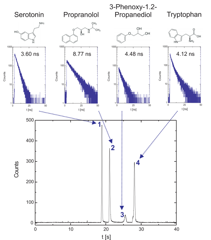
 Time-resolved fluorescence microscopy in the deep UV can be employed in microfluidic environments and enables label-free detection and identification of various aromatic analytes in chip electrophoresis. The results show the electrophoretic separation of a mixture of small aromatics (188 µm Serotonin, 135 µm propranolol, 238 µM 3-phenoxy-1.2-propanediol and 196 µM tryptophan). Fluorescence decay curves are gathered on-the-fly and average lifetimes can be determined for different substances in the electropherogram with the aim to identify aromatic compounds in mixtures. Based on the Time-Correlated Single Photon Counting the background fluorescence can be discriminated resulting in improved signal-to-noise-ratios. In addition, microchip electrophoretic separations with fluorescence lifetime detection can be performed with protein mixtures emphasizing the potential for biopolymer analysis.
Set-up:
Reference: R. Beyreiss, et.al., Electrophoresis 2011, 32, 3108-3114
Using time-resolved fluorescence microscopy in the deep UV to detect NATA in a microfulidic environment
 10 µM NATA (N-acetyl-L-tryptophanamide) dissolved in water excited at 280 nm. The fluorescence emission at 350 nm was detected through an f/3.2 monochromator set to 16 nm bandpass. 1.3 million counts were collected within 60 seconds, corresponding to an average detection rate of 21.7 kHz, i.e. less than 1% of the excitation rate thereby avoiding pulse pileup effects. The measured instrument response function (IRF) has a FWHM of 700 ps. The picture shows the IRF (red), the decay (blue) and the fitted single exponential curve (black). The fitted lifetime is 2.88 ns and the reduced chi-square = 1.065. The quality of the results can be also judged by the residual distribution plotted at the bottom.
Set-up:
- FluoTime 200
- Excitation: PLS 280, 2.5 MHz repetition rate
- Analysis: FluoFit (replaced by EasyTau 2)
Latest 10 publications related to Time-resolved Fluorescence
The following list is an extract of 10 recent publications from our bibliography that either bear reference or are releated to this application and our products in some way. Do you miss your publication? If yes, we will be happy to include it in our bibliography. Please send an e-mail to info@picoquant.com containing the appropriate citation. Thank you very much in advance for your kind co-operation.